
Direct Detection of Solar Angular Momentum Loss with the Wind Spacecraft
TL;DR
I was lucky to be given the opportunity to work with AWESoME Stars at the University of Exeter during the summer between my 3rd and 4th years there. I worked under Prof. Sean Matt and Dr. Adam Finley to obtain a direct measurement of the angular momentum loss rate of the Sun using data from the Wind spacecraft. My specific role was to analyse the data to produce the measurement with guidance from the others on the team. The results were written up by Adam and published in the Astrophysical Journal Letters as Direct Detection of Solar Angular Momentum Loss with the Wind Spacecraft.
The information on this page is from the report which I wrote detailing the work I did personally. To read a full discussion of the science, please refer to the paper itself.
Introduction
The Sun is the closest star to us, the only one whose stellar wind is directly measurable. Our knowledge of our star is used as a reference for how we expect other stars in the universe to behave. It is difficult to understand a process in other stars if it is not first understood in the Sun.
The solar wind is an example of something which is not completely understood. It is a stream of charged particles, consisting mostly of protons and electrons from the ionisation of hydrogen, and alpha particles from the ionisation of helium during fusion within the Sun. This wind doesn’t travel at one average speed, rather it travels in one of two types of stream; fast and slow. Slow wind is not fully understood, but it is known that it has conditions resembling those at the Sun’s corona with an average speed of 400 kms\(^{-1}\), and originates from areas of the Sun with closed magnetic field lines. The fast wind is better understood, at an average speed of 700 kms\(^{-1}\). Its conditions match those of the Sun’s photosphere, and it originates from coronal holes and areas of open flux. Through the solar wind, the Sun loses approximately 10\(^{12}\) gs\(^{-1}\), and this mass carries with it angular momentum.
Over the lifetime of a star, its rotation about its axis will change significantly. During periods of contraction, such as during its formation, conservation of angular momentum causes the rotation to speed up. While on the main sequence however, angular momentum can be lost due to particles in the stellar wind carrying angular momentum away from the Sun, as well as stresses in its own magnetic field applying a torque.
Multiple methods of estimating the angular momentum loss of the Sun use models to predict a value. Each method yields a different result. Without an experimental value to work towards, it is impossible to know which of these models is the most accurate.
This project aims to produce a value for the rate at which the Sun is losing angular momentum.
Open flux
The angular momentum flux of the Sun can be calculated theoretically. Magneto Hydrodynamic (MHD) models can be used to obtain a value, and there are many methods of doing so. One such method uses the open flux.
The open flux, the flux along the open field lines in the solar magnetic field, can be related to the Alfvén radius. This is the radius at which the bulk velocity of the waves in the magnetic field equals the Alfvén velocity (Belenkaya et al., 2014). This radius is important, as mathematically, the stresses in the magnetic field exert the torque required to produce co-rotation at the Alfvén radius (Weber and Davis, 1967), though this does not happen physically. Knowing this distance, it is possible to calculate the torque on the Sun due to the magnetic stresses.
Open flux is defined as \begin{equation} \label{eq:flux_integral} \phi=\int\mathbf{B}\cdot d\mathbf{s}. \end{equation} By evaluating the integral over the surface of a sphere, the open flux can be calculated using
\[\phi_{open}=4\pi \langle R^2 |B_r|_{hr} \rangle_{27 days}\]by assuming that the field lines at this radius will be predominantly open. The magnetic field is taken in one hour cadence in order to reduce small time-scale fluctuations before taking the modulus.
Using this value, the magnetisation parameter can be calculated as \begin{equation} \label{eq:magnetisation} \Upsilon_{open} = \frac{\phi_{open}^2 / R_*^2}{\dot{M}v_{esc}}, \end{equation} where \(R_*\) is the solar radius (\(6.96\times10^{10}\)cm) and \(v_{esc}=\sqrt{2GM_*/R_*}\) with \(M_*\) being the solar mass \(1.99\times10^{33}\) g. \(\dot{M}\) represents the mass loss: \begin{equation} \label{eq:mdot} \dot{M}=4\pi\langle R^2 v_r \rho\rangle_{27 days}. \end{equation}
The magnetisation parameter can be used to obtain the average alfvén radius:
\begin{equation} \label{alfven} \frac{\langle R_A \rangle}{R_*} = K_o[\Upsilon_{open}]^{m_o}, \end{equation}
where \(K_o=0.33\) and \(m_o=0.371\) (Finley and Matt, 2018) which then allows the torque due to the solar wind to be calculated as
\[\tau = \dot{M}\Omega_*R_*^2 \left( \frac{\langle R_A \rangle}{R_*} \right) ^2.\]Here \(\Omega_*\) is the solar rotation rate, \(2.6\times10^{-6}\) rads\(^{-1}\).
This value for the torque can then be compared to that produced via the other three methods, and with the result from the Wind data arrived at in this report. Previously, a value of \(2.28\times10^{30}\) erg was obtained using data from the Ulysses and ACE spacecrafts by Finley et al., 2018.
Data Analysis
Coordinate Transformations
The particle and field data from Wind is initially given in Geocentric Solar Ecliptic (GSE) coordinates, a cartesian system which defines the x-axis as the direction of the Sun from Earth, the z-axis as the Earth’s ecliptic north pole, and the y-axis as perpendicular to both such that it forms a right handed coordinate system.
In order to measure the solar angular momentum flux, however, it is convenient to use Radial, Tangential, Normal (RTN). This is a heliocentric cartesian coordinate system defining X as the line connecting the Sun to the spacecraft, Y as the cross product of the solar rotational axis and X, and Z as perpendicular to both.
Removing Erroneous Data
Not all data from the Wind spacecraft was usable. First, there were many empty values, denoted by an impossible value such as 99999.99 or similar, which had to be removed. If either a component of proton velocity or density was empty, the complete set of data for that observation time was removed. This was because the angular momentum calculation required all the proton values to be correct. Alpha particle values were more frequently empty, and when this was the case the proton data was saved, removing only the alpha velocities and density.
| Flag | Meanings |
|---|---|
| 10 | Solar wind parameters OK - no action necessary |
| 9 | Alpha particles are relatively too cold |
| 8 | Alpha particles overlap within protons in current distribution function |
| 7 | Alphas too fast, out of SWE range |
| 6 | Alpha particle peak may be confused with second proton peak |
| 5 | Parameters OK, but Tp=Ta constraint used (params obtained with SUB_PROT=1) |
| 4 | Alphas are unusually cold, Tp=Ta constraint used (SUB_PROT=1) |
| 3 | Alphas are relatively too hot (SUB_PROT=1). Tp=Ta constraint used |
| 2 | Alphas are unusually slow |
| 1 | Poor peak identification |
| 0 | Spectrum cannot be fit with a bimax model. May be strongly non-Maxwellian or may contain a discontinuity |
Next, the data had to be filtered according to the flags, described in the table above. The alpha particles were prone to issues and the focus of most of the flags. Therefore, the alpha data was removed if it did not correspond with a flag of 10, meaning the parameters were fine. For the protons, most of the flags had little effect. Only data with flags of 1 or 0 had to be removed. If this was not done, the angular momentum loss was often negative, especially during solar minimums.
The removal of most alpha particle data is an issue. In order to obtain a value for the total angular momentum flux at any moment, values for all components are needed. The fact that the data was flagged does not mean there is no alpha component, so a method for reintroducing alpha particles into the data is needed. Since most issues with the alpha particles are due to their peaks being difficult to separate from those of the protons, it is assumed that their speeds were similar. Thus, their velocities are approximated to be equal to those of the proton data at that time. Alpha number densities are approximated to 4% of that of the protons (Borrini et al., 1983).
Interplanetary Coronal Mass Ejections
The aim of this project is to obtain a value of the solar angular momentum loss due to field stresses and the ambient solar wind. Interplanetary Coronal Mass Ejections (ICMEs) are bursts of plasma originating from an event on the Sun’s corona. They are expected to have little effect on the global angular momentum loss, and since they are a type of local fluctuation, they should be removed from the data.
Initially, ICMEs are removed from by placing upper limits on the particle densities and magnetic field strengths. If the proton density at a certain time exceeded this value, none of the values at that time are included in the averages. The first value attempted is a limit of 10 nT for the field and 10 m\(^{-3}\) for the proton and alpha number densities.
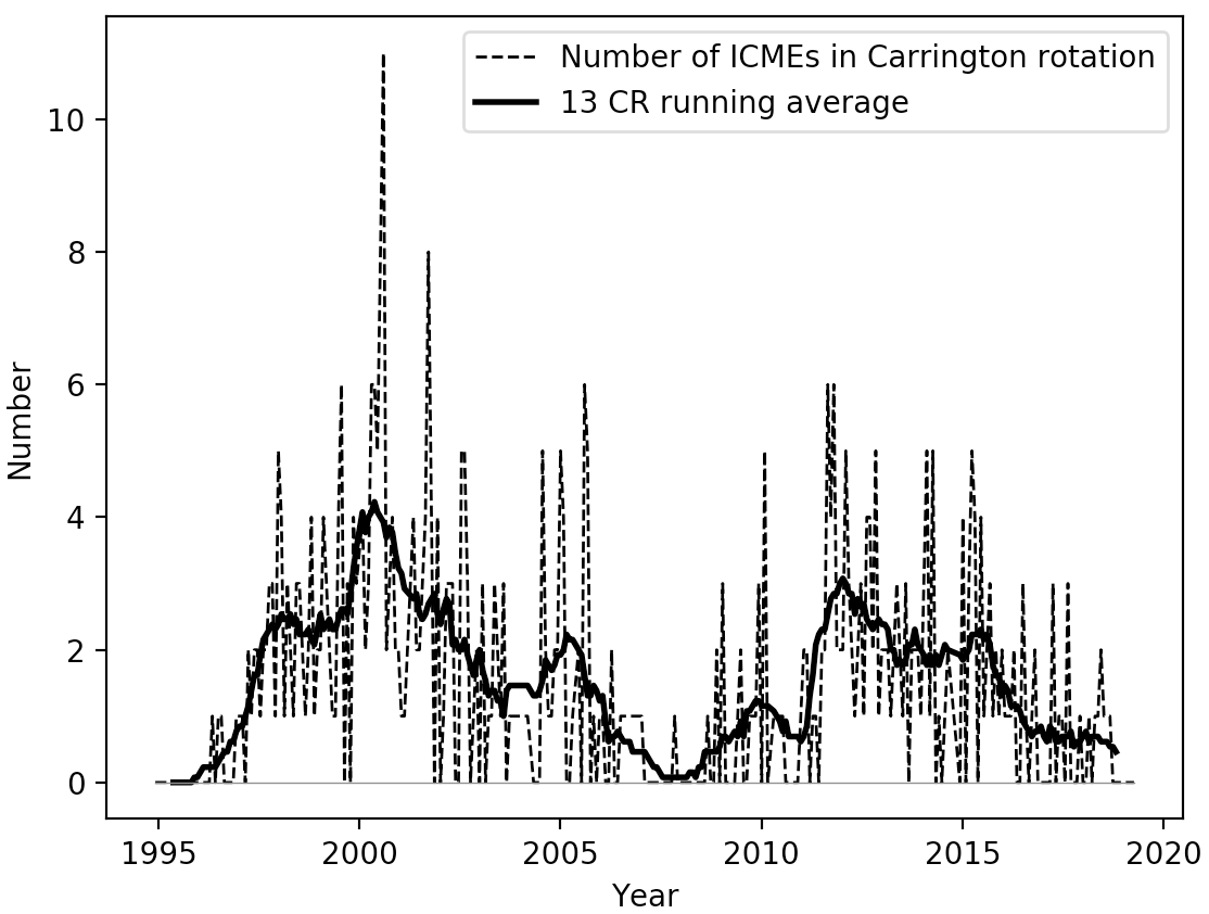
This method appears to be removing too much of the data however, so the Cane and Richardson ICME list is used instead. The number of ICMEs per Carrington according to this list can be seen in Figure 1. The list gives the start times of the shock and the end times of the trailing edge of each ICME since May 1996, so data taken between any of these two times is removed.
For the period which is not covered by the Cane and Richardson ICME list, another method of filtering the data is required. By comparison by eye of different conditions to the data with the ICMEs removed according to the list, a best fit is obtained; 30 nT for the field and 70 m\(^{-3}\) for the proton and alpha densities.
Averaging the Data
A Carrington rotation (CR) is the length of time it takes for a sunspot to travel the circumference of the Sun and return to its original location as viewed from the Earth. It is roughly 27 days long, meaning there are 13 of them in a year.
Raw data from Wind has a varying cadence of around 2 minutes, though this can vary massively. Carrington rotation averages are taken so that each value would represent an average across the whole solar equator. From this value, a profile for the Sun can be used to obtain an average value across the whole solar surface.
Averages are taken after calculations with the values were made at the 2 minute cadence. If, once data had been processed according to the methods above, there are fewer than 10,000 data points in one Carrington rotation (around 50% of the data points remaining), that rotation is removed and not plotted.
Results
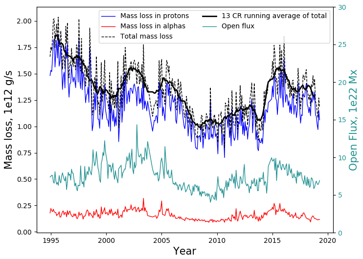
The global mass flux is shown in Figure 2. The blue and red lines represent the mass flux in the proton and alpha particles respectively. Their total is plotted in dashed black, while solid black shows a smoothed 13 CR average. The open flux, shown in teal, is representative of solar activity, being greater at solar maxima. The alpha contribution shows a clear correlation with solar activity while the protons show a much more complicated relationship. The mass loss of the Sun has been plotted before and so can be compared to determine whether the data is being handled correctly. The mass flux is calculated from values which are measured reliably by most spacecraft, so results should be similar. Figure 1 in Finley et al., 2018 shows the mass flux from ACE and Ulysses spacecrafts. From Figure 2, it is clear that the majority of the mass flux is due to the protons.
Azimuthal Velocities
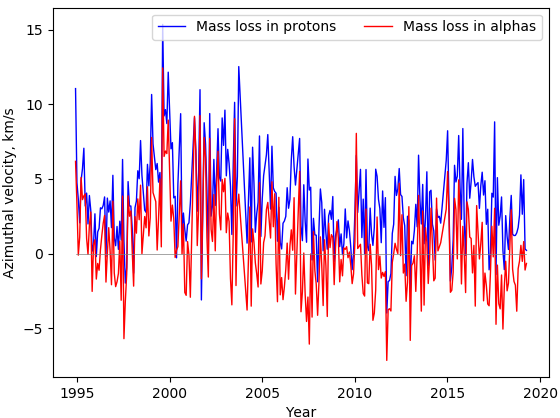
The azimuthal velocities (\(v_t\)) of protons and alpha particles are shown in Figure 3 in blue and red respectively. Each point represents the average azimuthal velocity in that Carrington rotation, weighted by number density using \(v_t=\frac{\langle v_t \rho \rangle_{CR}}{\langle \rho \rangle_{CR}}.\) The azimuthal velocity represents the component of velocities that carries angular momentum, therefore it is crucial to accurately measure it. However, it is often on the order of kms\(^{-1}\), which makes it hard to separate from the 400 kms\(^{-1}\) of the radial component. From the graph, it is evident that the azimuthal component of the wind fluctuates to a level comparable to the average value. This makes the accuracy of the measurement all the more important. Many spacecraft experience problems here, making it impossible to calculate a useful value of angular momentum flux. This issue is compounded when the spacecraft also has a pointing error, such as the Helios spacecraft. Wind does not have a pointing error, and its azimuthal velocities are good. At the time of writing, it is one of only two spacecraft which are capable of calculating a value of solar angular momentum loss, along with IMP8.
Discussion
Wind Stream Interactions
Fast wind has been observed to contribute negative angular momentum flux, likely due to interactions with the slow wind. Slow wind is the majority of the wind, any fast wind will collide with the slow wind once far enough from the Sun. When this happens, the two winds exchange momentum; the slow wind will be accelerated in the direction of co-rotation and the fast wind will be oppositely affected. Since the fast wind is less dense than the slow wind, its acceleration will be greater.
Weak Alpha Particles
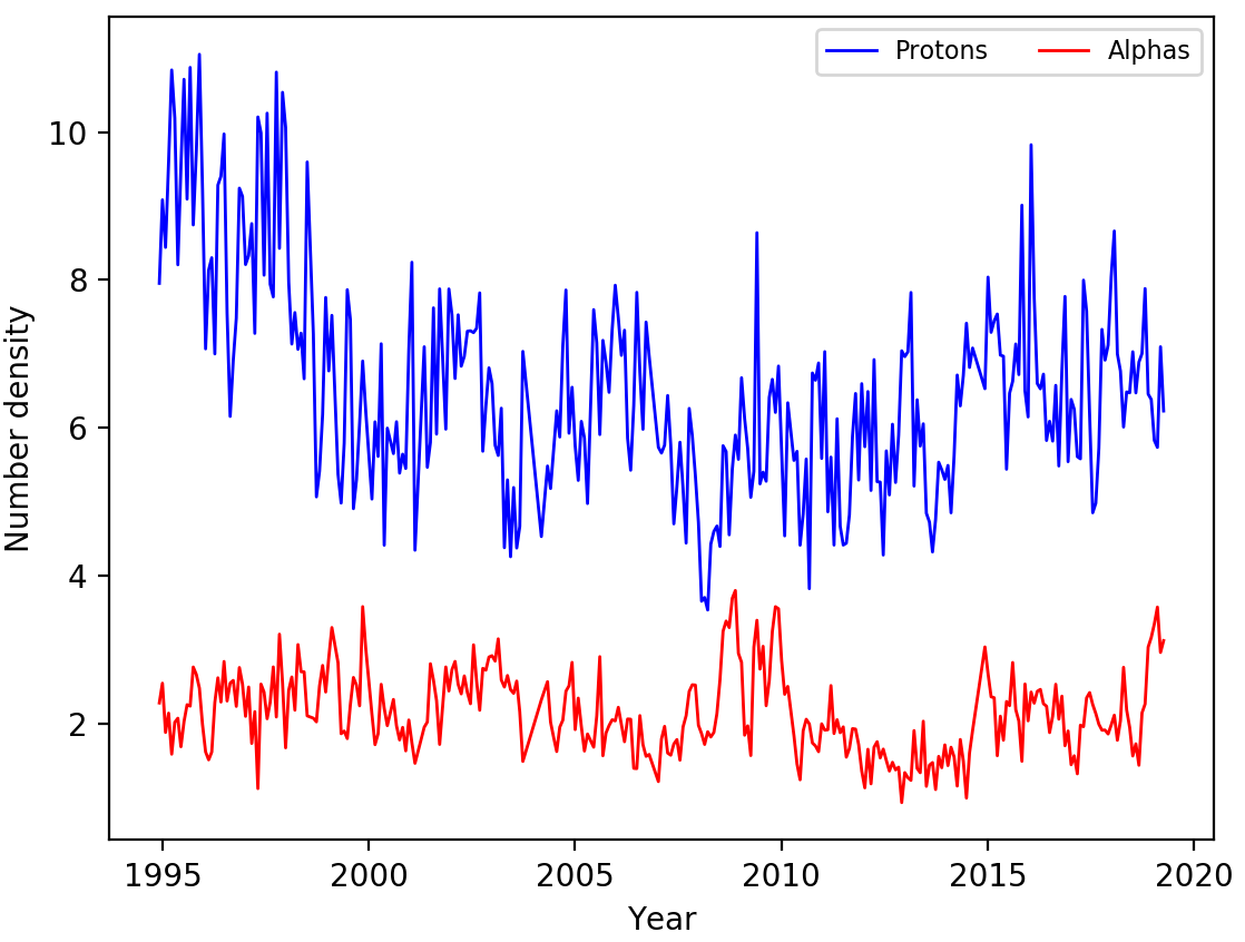
The protons may dominate due to reduction of the alpha particles during the data analysis stage. As shown in Figure 4, the velocities of the alpha particles and protons are not equal as assumed during the data analysis. The assumption that the velocities are equal is based off the error being caused by the velocities being too similar for the alpha and proton to be separated. However, this may not always be the case, and may prevent the alpha contribution being more negative.
Additionally, the assumption that the density of the alphas is 4% the density of the protons may reduce the alpha contribution more than in reality. Figure 4 shows the average number density per CR after this assumption has been used on the missing alpha particles. The lack of reliable alpha data makes comparison between proton and alpha particles using the Wind data difficult.